trackers package
Submodules
trackers.tracker module
Equations of Motion
| Authors: | Helga Timko |
|---|
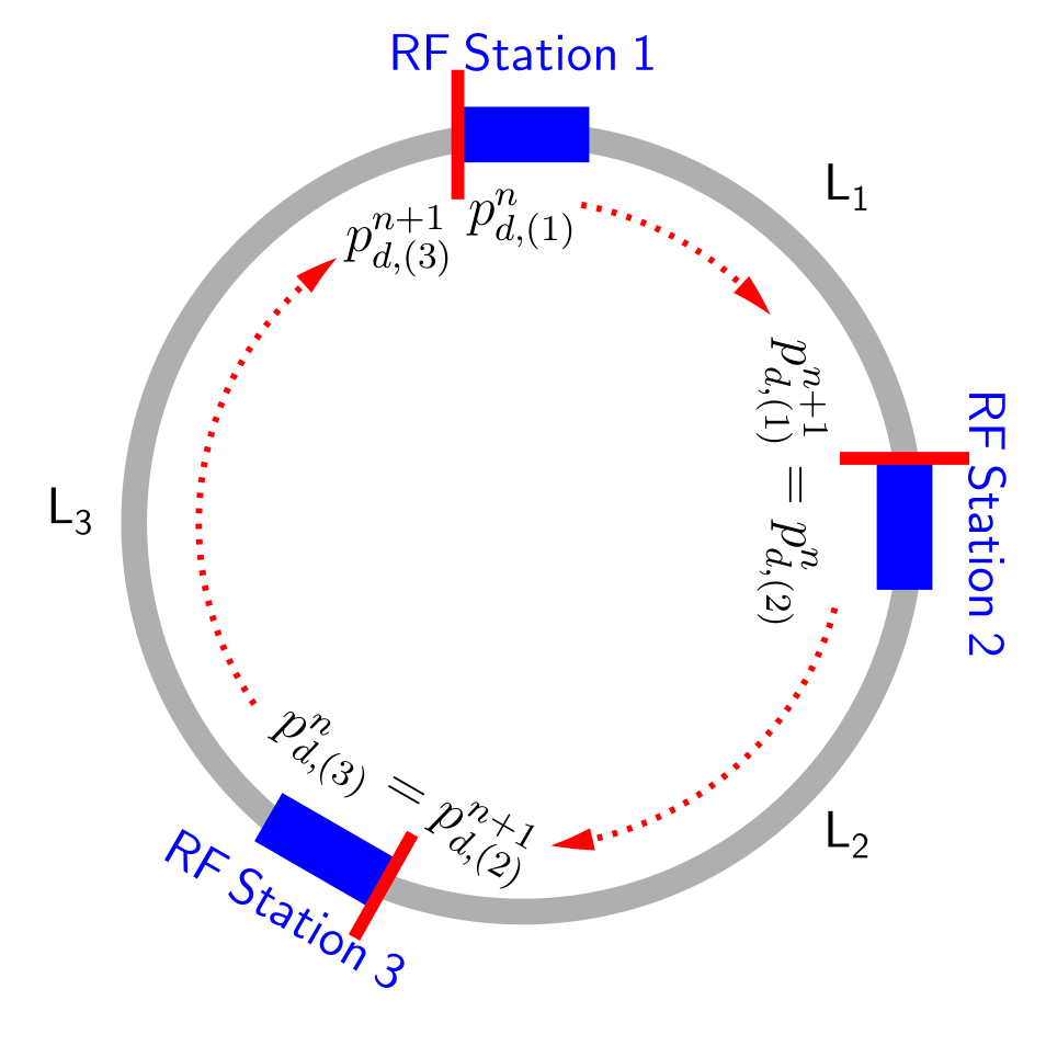
Below, we shall derive the equations of motion (EOMs) for an energy kick given
to the particle by the RF caviti(es) of a given RF station and the subsequent
drift of the particle during one turn, see Figure. In the case of multiple RF
stations, the drift equation should be scaled by  , where
 is the machine circumference.
Definitions
Code-internal units are SI-units unless otherwise specified in the below table.
| Code-internal units: | |
|---|---|
Energy Momentum Mass Time Frequency Angular frequency |
|
 = [eV]
 = [eV]
 = [s]
= [s] = [Hz]
 = [rad/s]
Just like in the real machine, we demand the user to define beforehand the
energy programme, i.e. the synchronous (design) total energy at every time
step  and RF station
  ,
,  .
This will define the design momentum
.
This will define the design momentum  through following relations:
(1)
(2)
(3)
where  is the mass of the particle, and energy, momentum, and mass are
given in [eV].
is the mass of the particle, and energy, momentum, and mass are
given in [eV].
For a given synchronous orbit with an average radius  , the
angular frequency will be
, the
angular frequency will be  and one
turn will take
and one
turn will take  at the synchronous
energy. The magnetic field programme is assumed to be synchronised with the
design energy turn by turn. Hence, a particle leaving the RF station with the
synchronous energy will always be on the synchronous orbit and return to the RF
station after exactly one period, unless the actual magnetic field differs from
the designed one.
at the synchronous
energy. The magnetic field programme is assumed to be synchronised with the
design energy turn by turn. Hence, a particle leaving the RF station with the
synchronous energy will always be on the synchronous orbit and return to the RF
station after exactly one period, unless the actual magnetic field differs from
the designed one.
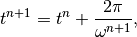
We define then an external reference (clock) time
(4)
and as initial condition we choose the sinusoidal RF wave of the main RF
system (harmonic  and RF frequency
  )
to be at phase zero at time zero:
)
to be at phase zero at time zero:
(5)
All phase offsets of all RF systems are defined w.r.t. this initial condition
and w.r.t. to the main RF system. Phase offsets can be programmed through the
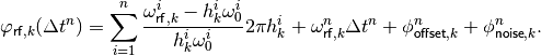
phi_offset parameter. In addition, RF phase noise
 can be added through
 phi_noise for each
system. For  RF systems in the RF station the total
voltage [eV] becomes:
RF systems in the RF station the total
voltage [eV] becomes:
(6)
We define the arrival time of an arbitrary particle to the RF station relative to the reference time in that turn,
(7)
The total phase offset at the reference time is tracked in the variable
phi_RF, defined through
(8)
Energy kick
During the passage through an RF station, the energy  of an
arbitrary particle is changed by the total energy kick received from the
various RF systems in the station. The energy change due to the induced
electric fields in the magnets is negligible and beam-induced voltage is taken
into account in the
of an
arbitrary particle is changed by the total energy kick received from the
various RF systems in the station. The energy change due to the induced
electric fields in the magnets is negligible and beam-induced voltage is taken
into account in the impedance module. The phase of the RF voltage of system
k at the arrival time  of any particle is:
(9)
Subtracting multiples of  , which can be neglected,
(10)
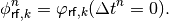
Note that phi_RF is determined through the above equation,
(11)
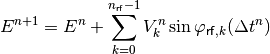
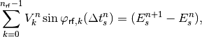
Thus the total energy change equation is
(12)
Note
Eq. (12) is intrinsically discrete; no approximation has been done.
Note
The RF phase (Eq. (11)) differs from the sum of phase offset
and phase noise only if the RF frequency differs from the design RF frequency
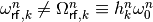 ,
i.e. when feedback loops are active.
,
i.e. when feedback loops are active.
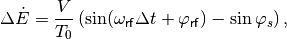
Rather than the absolute energy, we are actually interested in the energy
offset of a given particle w.r.t. the synchronous energy
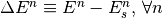 . So we choose our
coordinate system to be centred around
. So we choose our
coordinate system to be centred around  . Substracting
 from both sides of Eq. (12), we arrive at
(13)
Warning
As a consequence, during acceleration the coordinate system is non-inertial and a coordinate transform is done turn by turn.
Arrival time drift
The frequency slippage of an off-momentum particle during one turn is defined w.r.t. the design synchronous particle,
(14)
where 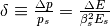 is the relative off-momentum of the particle and
  are the
slippage factors
are the
slippage factors
(15)
which are defined via the momentum compaction factors  .
.
The absolute arrival time of an arbitrary particle can be expressed as a recursion
(16)
with initial condition  and where the revolution frequency of
the particle
and where the revolution frequency of
the particle  can differ from
 due to energy and orbit deviations from the synchronous
particle.
due to energy and orbit deviations from the synchronous
particle.
Note
Eq. (16) contains  as we chose to perform
the energy kick first and the subsequent time drift happens according to the
already updated energy.
as we chose to perform
the energy kick first and the subsequent time drift happens according to the
already updated energy.
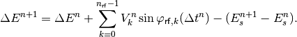
Using Eq. (7), the recursion on the particle arrival time relative to the clock becomes
(17)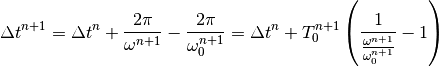
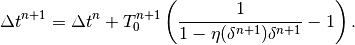
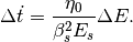
Using definition (14), the arrival time drift can be calculated as
(18)
If a zeroth order slippage is used,  , the
option
, the
option solver = 'simple' can be used to approximate the above equation as
(19)
The synchronous particle
A particle is synchronous in turn n if it enters and leaves the RF station
with zero energy offset,  , and thus
gains exactly the designed energy gain
, and thus
gains exactly the designed energy gain  . As a
consequence, in the absence of induced voltage the synchronous particle will
fulfil:
. As a
consequence, in the absence of induced voltage the synchronous particle will
fulfil:
(20)
and in the presence of intensity effects, the induced voltage from the particles in front should be added on the left-hand side:
(21)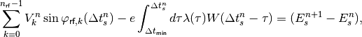
where  is the beam/bunch profile and
  the wake
potential.
the wake
potential.
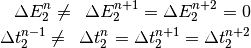
Warning
In general, these equations have
solutions. If the synchronous energy gain changes
from one turn to another, also the synchronous particle changes with it.
Note
Synchronous particle arrival time
As a consequence, the arrival time of the synchronous particle
 is not necessarily constant, but can change from turn to
turn. This might be counter-intuitive, as the synchronous particle drifts
with exactly
is not necessarily constant, but can change from turn to
turn. This might be counter-intuitive, as the synchronous particle drifts
with exactly  along the ring. To see this effect, consider
two subsequent turns with different synchronous energy gains
along the ring. To see this effect, consider
two subsequent turns with different synchronous energy gains
 in a single-RF system.
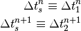
Let particle 1 be synchronous in turn n and particle 2 be synchronous in
turn
in a single-RF system.
Let particle 1 be synchronous in turn n and particle 2 be synchronous in
turn  :
:
(22)
(23)
The arrival time of the synchronous particles in this case will be:
(24)
Thus, because the synchronous particle can be a different particle each turn, the recursion on the synchronous arrival time becomes in general
(25)
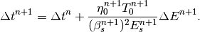
The difference in arrival time of the two particles in turn n can be determined from the energy equations
(26)
which in first-order approximation (see Small-amplitude oscillations) gives
(27)
Small-amplitude oscillations
Assuming a single-RF station and a simple solver (Eq. (19)), the EOMs in continous time can be written as
(28)
(29)
Assuming further a constant synchronous phase
 and expanding the RF wave
around it
and expanding the RF wave
around it
(30)
we obtain for the sinusoidal term in first order
(31)
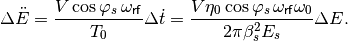
Derivating Eq. (28) a second time, and using Eq. (29)
(32)
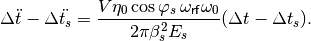
Vice versa, derivating (29) another time, and substituting
Eq. (28), an equivalent equation can be found for the arrival time w.r.t.
to the arrival of the synchronous particle :
(33)
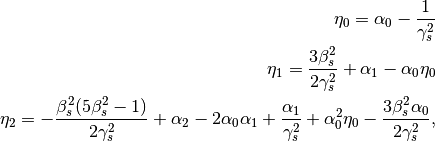
Equations (32) and (33) describe an oscillating motion in phase
space if  , which for
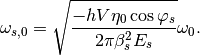
 has the synchrotron frequency
(34)
Note
that energy and time are conjugate variables, whereas energy and
phase are not. When forming time derivatives in phase, one should take into
account the frequency correction from one turn to another:
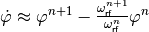 .
.
trackers.utilities module
Tracking utilities
| Authors: | Helga Timko |
|---|
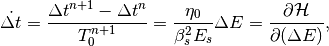
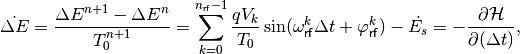
Hamiltonian
To construct the Hamiltonian  from the conjugate variables
 and
and  , let us first rewrite the equations of
motion in continuous time (for a zeroth-order slippage factor):
, let us first rewrite the equations of
motion in continuous time (for a zeroth-order slippage factor):
(35)
(36)
from which we obtain the Hamiltonian by partial integration:


The constant of integration can be chosen such that

from which the Hamiltonian becomes

In case of a single-harmonic RF system with
, the second term can be replaced
with  , and we obtain the know
textbook formula
, and we obtain the know
textbook formula

or in terms of particle phase  ,
,

Separatrix
To construct the separatrix, first the unstable fixed point (UFP) needs to be
determined. Its coordinates  are
calculated numerically by looking for the smallest (largest) zero crossing
position in one period of the total voltage waveform above (below) transition.
The separatrix is the equipotential line that goes through the UFP and is thus
defined by the condition
are
calculated numerically by looking for the smallest (largest) zero crossing
position in one period of the total voltage waveform above (below) transition.
The separatrix is the equipotential line that goes through the UFP and is thus
defined by the condition

Solving this equation we obtain
![\Delta E_{\mathsf{sep}} = \pm \sqrt{ \frac{2 \beta_s^2 E_s}{\eta_0} \left \{ \sum_{k=0}^{n_{\mathsf{rf}}-1} \frac{q V_k}{T_0 \omega_{\mathsf{rf}}^k} \left [ \cos (\omega_{\mathsf{rf}}^k \Delta t_{\mathsf{ufp}} + \varphi_{\mathsf{rf}}^k) - \cos (\omega_{\mathsf{rf}}^k \Delta t_{\mathsf{sep}} + \varphi_{\mathsf{rf}}^k) \right ] + \dot{E_s} (\Delta t_{\mathsf{ufp}} - \Delta t_{\mathsf{sep}}) \right \}} .](_images/math/b6afdf20d0cd534cc3eb5b7713a81743709dda62.png)
In the case of a single-harmonic RF system with
, the phase of the UFP is
 . In addition,
, so the above equation reduces to
. In addition,
, so the above equation reduces to
In practise, to calculate the separatrix for input arrays
 that are longer than the period of the voltage
waveform, the routine takes into account periodicity and projects the input
array onto the ‘basic period’ of the waveform (that is
that are longer than the period of the voltage
waveform, the routine takes into account periodicity and projects the input
array onto the ‘basic period’ of the waveform (that is  and
and
 on the first harmonic, below and above transition,
respectively).
on the first harmonic, below and above transition,
respectively).